Hybrid Algorithm for Interpolation Based on Macro-block Gray Value Gradient under H.264

H.264 standard is a new generation video compress standard composed of ITU-T and ISO/IEC, which supports multi-frame selection and up to 7 motion estimation modes, consequently [1][ 2]. Andmotion estimation takes a larger computation in H.264 coders. Various searching algorithms which are applied to reduce the motion estimation could be divided into: (1) Full Searching (FS) reducing load of searching by assistance strategy. For instance, choosing a dynamic searching centre or jumping out the matching searching in advanced to reduce the calculation for block matching, and so on. (2) Partial Searching utilizing reduction of searching forthe spatial position candidates or special principle for matching. But the faults of them are the calculation is too complex, the calculation quantity is too large. So the improvement of motion search algorithm based on blocks looks rather important. The improvement is mainly modified from the following three faces: the choice of initial search points, the matching rule and the search strategy. Numerous scholars produce lots of new Fast Integer Motion Search, mainly including three steps method, altogetherclutches the direction search method, Two-dimensional algorithm drop method, four steps method, Diamond method and so on [2]. The improved algorithm produced in this paper mainly improves efficiency of algorithm from search strategy, and then reduces search time of the motion estimation.Accepted February 18, 2009The value derived from bilinear interpolation depends on average sum of 4 adjoined grid points. In another word, it is based on distance between the interpolated pointand neighbor points to decide the corresponding weights and compute interpolation value ultimately. For linear function interpolation, function f ( x ) defined within the rectangle N should be taken into consideration, the formula is: f (x) = ∑ h(x,n)f(n) n ⊂ N (1) x is a point among the region of N , h ( x , n ) is the linear interpolated weight function. A typical interpolated weight function is Lagrange polynomial: h (x ,n )= ∏ i ≠ n n x − − i i (2) The linear interpolated weight function of Equation (2) changes into: h (x ,n )= { 1 0 - x -n n + n 1 -1 ≤ < x x o < r x n ≤ + n 1 -1 (3) H.264 applies a Wiener filter to complete interpolation for positions of half-pixels, and further to get quarter pixels precision by bilinear interpolation. As shown in Fig.1, capitals A, B, C, D are entire pixels. b, h, m, s and aa, bb, gg, hh are half-pixels gained
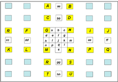
   by the Wiener filter. The rest quarter-pixels of
a , c , d , n , f , j , k , q are gained through interpolation between entire pixels and neighbor half-pixels. [Fig.1] Pixel positions The formulas are as following: a = ( G + b + 1) >> 1 i = ( h + j + 1) >> 1 c = ( H + b + 1) >> 1 c = ( b + j + 1) >> 1 d = ( G + h + 1) >> 1 k = ( j + m + 1) >> 1 h = ( M + h + 1) >> 1 q = ( j + s + 1) >> 1 (4) The others: e = ( b + h + 1) >> 1 p = ( h + s + 1) >> 1 g = ( b + m + 1) >> 1 r = ( m + s + 1) >> 1 (5) From the equation above, to obtain a quarter-pixel interpolation, 2 addition and 1shift compute are needed. Even though the whole procedure is simple, the frequency spectrum of bilinear interpolation is similar to a low-pass filter, which leads to an incorrect interpolation for high-frequency signals. However, it is right high-frequency signals that reflect edge information in images mostly, hence the edge information of the image is weakened under such situation and image turns to be relatively blurred. Cubic interpolation is also widely applied in numerical analysis besides bilinear interpolation. According to interpolation theory [6], 2-Dimention image cubic interpolation of even-interval samples can be presented as3. Cubic Interpolation and Applications in H.264
   following: S ( x , y ) = ∑∑ C ( x 1 , y m ) h (| x − x 1 |) h (| y − y 1 |) 1 m (6) Where s ( x , y ) is defined as interpolated point,
c ( x 1 , y m ) , sample value of pixel ( x 1 , y m ) , and h is the function for interpolation weights. The selection of h is the core of Cubic interpolation. Single-variable interpolation weight Selection in H.264 mainly lies on Coons – Gordon surface, which is a bi-variable interpolation could be constructed by an approximately repeated single-variable interpolation. Single-Variable Cubic interpolation core value [ 3]: ⎧ ( A + 2) ⋅ x 3 − ( A + 3) ⋅ x 3 + 1 0 ≤ x < 1 h ( x ) = ⎨ ⎪ A ⋅ x 3 − 5 A ⋅ x 3 + 8 A ⋅ x − 4 A 1 ≤ x < 2 ⎩ ⎪ 0 (7) Practically, A is chosen to be 1/2. In Cubic interpolation utilized in image processing, it is necessary to expand a one-dimension Cubic interpolation to a 2-dimension Cubic interpolation, and then take use of equation(5), picking up the 4-by-4 pixel close to the pixel to be detected for interpolation. a = F b = 0.5625( F + G ) - 0.0625( E + H ) c = 0.5625( F + J ) - 0.0625( B + N ) d = 0.0625 × 0.0625( A + D + M + P ) + 0.5625 × 0.5625( F + G + L + (8) K ) − 0.5625 × 0.0625( F + G + L + K )( B + C + E + I + H + L + N + O ) Generally, Cubic interpolation possesses wider frequency-band than that of the bilinear method [4][5]. Besides, it preserves the high-frequency parts generating higher precision but more complex in calculation. In mathematics, bilinear interpolation is an extension of linear interpolation for interpolating functions of two variables on a regular grid. The key idea is to perform linear interpolation first in one direction, and then again in the other direction. Bicubic interpolation is an extension of cubic interpolation for interpolating data points on a two dimensional regular grid. The interpolated surface is smoother than corresponding surfaces obtained by bilinear interpolation or nearest-neighbor interpolation. Compared with the two algorithms discussed above, bilinear interpolation is very effective to Low-frequency signals (the regions where gray-values distribute regularly) besides not being so computational, cubic convolution is acting on high-frequency parts (the regions where gray-value distribute irregularly), especially on protecting the edge regions of images, but it is rather computational. To balance theinterpolation precision and complexity, a good trend is proposed as to pick up different interpolation according to gray-value characteristics in different parts of blocks. Grounded on statistical theory, square difference can be used as a threshold to judge the regularity of gray-value distribution in a block. However, it requires large amount of computation on all the pixels in the blocks according to: S ^ = ∑ X * X / N (9) In the other hand, the edge parts of images which is the most effective to human’s vision concentrates in a certain part of a block, where cubic interpolation or some other high-precision algorithms are adopted; while in other parts where gray-values distribute regularly, bilinear interpolation is good enough. So this simple selection principle combines the strong points of both bilinear and cubic interpolation. In each block, distance between two neighbor pixels is certainty. To equal-interval sampling data, an interpolation can be represented as:4. Selection of Proper InterpolationWhere is an interpolation kernel, is weight coefficient, is the number of data used for convolution. As a matter of fact, is always symmetric in practical, that is to present h ( x ) = h ( − x ) , is the sampling value. From (9), it is clear that when takes different functions, the interpolation result will be different, so the algorithm alters. Actually, we can infer that:Regardless of which kind of function is being applied. Evidently, if the gray-values of reference points are equal, then the gray-value of the interpolated points will be the same with that of reference ones, generating no changes judging by human eyes. So if we want to produce obvious changes which could be perceived by naked eyes, it is necessary to make a step-change between the interpolated points and reference point in adjacency. The stronger the changes produce stronger vision perception. Suppose that an interpolated point’s gray-value is f ( x ) the changing gradient is
   C k is a weight coefficient, and A ( x k ) is a gray-value
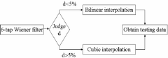
adjoining to point with gray-value equal to f ( x ) . From the equation (11), we can find that weight coefficient and the selection for the numbers of adjacent points are crucial to the precision of gradient d . Under H.264, during the procedure of searching for motion, the first interpolated value f ( x ) can be obtained through a 6-tap wiener filter. Taking computation complexity into consideration, we only take two integer pixels that are most close to f ( x ) . Take Fig.1 as an example, for point h we take the integer point G and M while for point b, G and H in horizontal direction will be picked up which is most closed in vertical direction, and C k is replaced by 1/2 here. When d< 5 %, the gray-value of F ( x ) does not change greatly, to which human’s eyes does not react sensitively enough. Approximately, assume the half-pixel found by motion search changes little compared with the adjacent gray-values. In practical, there is no much difference in result, whatever any algorithm adopted in second interpolation. The structure described details as following: Consequently, after the first interpolation of a block finishing finding the best matching pixels, if the gray-values of the pixels are consist to that of the neighborhood region, choosing bilinear algorithm for next interpolation; or else cubic method would be better. In this way, the results costs less time for computation without loss of interpolated quality in the meantime.[Fig. 2] Proposed algorithm5.1 Experiment Environment To validate the effecting form the algorithm proposed in this paper, we applied the Coding program supplied by TML-8, utilizing the interpolation algorithm proposed only for motion compensation parts. In our experiment, the standard test sequence "Miss American"was chosen as the source image, mostly on that it features for slow motion and comparatively simple. Each sequence adopts the format of QCIF 50fpr (176×144 Pixels, Y :U :V = 4:2:0), testing on a Pentium4 PC. During coding procedure, all the motion estimation applied matching-fit, based on SAD principle, Using Fast-Diamond searching for motion searching. Simultaneously, Fixed-Step strategy was used for removing the difference derived from the control by various code rates. The performance comparison between Bi-linear algorithm and the proposed algorithm was measured based on (Peak Signal-to-Noise) PSNR and compression ratio.PSNR is the average Peak value of SNR for multi-frame images, which is a significant metric for the entire coder. It is expressed as: (dB)
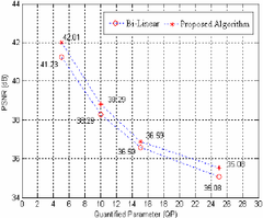
   Where the size of the image is M × N , L is the number of frame, of original image at the point of ( m , n ) , f k ( m , n ) is the pixel value of the k th frame in image. The difference between Bi-linear and proposed algorithm is shown in Fig.3.
[Fig. 3] Comparison of PSNR between Bi-linear and Proposed AlgorithmFrom the data shown in the Fig.3,with the increase of quantified parameters, the number of zero-block increases accordingly, hence, PSNR will decrease in a certain extent. While the quantified parameter of "Miss America image" sequence is 5, the PSNR obtained from a simple bi-linear interpolation will be raised to around 0.8 dB. As the quantified parameters increase, PSNR from both algorithm declines largely. However, the PSNR got from the algorithm proposed in this paper is obviously 0.2~0.6 dB higher than regular algorithm
   [Table 1] Length variety of code sequence from 2 typical algorithms under different Qp. (Unit: byte) Proposed Bi-Linear variety(%) Algorithm 5 47680 46513 -2. 4 10 21025 20779 -1. 2 15 12607 12510 -0. 8 25 8477 8196 -3. 3
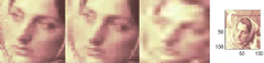
Before the both algorithms are selected, a Wiener filter must be used at first, so we skip this step here. After the judgment of the branch, the fit algorithm should be chosen. Fig.4 is the actual results of enlarged pictures. Each picture takes 25 samples, size of 100 ×100 pixels. Different algorithms are used to enlarge these pictures to 800 ×600 pixels. Experiment results just focus on the face part that contains many details.
   (a) (b) (c) (d) [Fig. 4] Experiment results of (a) Cubic interpolation, (b) the Interpolation of proposed method, and (c) Bilinear Interpolation Compared with Original picture (d)
Though one more offset judgment than single algorithm seems to increase complexity of the program, actually it equals to a single calculation, unparallel to computation cost by Cubic interpolation. From Fig. 4, it performed almost the same effecting with Cubic but much better than linear method. Obvious computation speed difference shows: the speed is raised up to 20%-30% when competed with utilizing Cubic interpolation alone. What is more, when judging on the ground of threshold, it quit automatically from searching once d is less than a certain extent, which also saves plenty of time for interpolation. The decision of exact value for threshold needs to be discussed.In this paper, we discussed a hybrid algorithm combining the advantages of Cubic and Bi-linear interpolation, against the limitation by using a single interpolation. Precision of gradient is adopted to judge the changes between the interpolated points and reference point in adjacency. Then the appropriate interpolation method will be chosen based on it. The results of our experiment proved it effective to improve image quality objectively and enhance the coding compress ratio, while brings no more coding consumption. Shi Wang [Regular Member] • 2000 ~ 2004 : Wuhan University of Technology, China, B.S. • 2004 ~ 2007 : Huazhong University of Science and Technology, China, M.S. • 2007 ~ Present : Div. of Electronics and Information Eng., Chonbuk National University, PhD. <Research Interests> Multimedia and Communications System, Segment-Based 3-D Matching, Robot Vision.Hongxin Chen [Regular Member] • 2000 ~ 2004: Wuhan University of Technology, China, B.S. • 2004 ~ 2007: Wuhan University of Technology, China, M.S. • 2007 ~ Present: Div. of Electronics and Information Eng., Chonbuk National University, PhD. <Research Interests> Multimedia and Communications System, Robot Vision, Remote Control.Hyeon-Joong Yoo [Regular Member] • 1982 ~ 1989:Researcher Agency for Defense Development • 1996: Senior Researcher, Industrial Electronics Dept., Samsun Co. • 1996 ~ Present: Dept. of Information and Telecommunication Eng. Sangmyung University.<Research Interests> Pattern Recognition, Image Processing, Neural NetworksHyongsuk Kim [Regular Member] • Jan. 1982 ~ Aug. 1992: Senior Researcher, Agency for Defense Development • May. 1992: University of Missouri, Columbia, PhD. • Sep. 1993 ~ present: Professor, Div. of Electronics and Information Eng., Chonbuk National University <Research Interests> Robot Vision, Sensors of Robots, Analog Parallel Processing System

References

- [1] Stockhammer T, Hannuksela M M,Wi – egand T. H.264 /AVC in Wireless Environments[J]. IEEE Trans, Circuits Syst, Video Technol, 2003, 13 (6): 657 -673.
- [2] I. Lille-Langoy, et al. Telenor. H.26L Proposal and Software ITU-T SG16/Q15doc. Q15-H-08 [S]. Berlin, 1999-08.
- [3] Schreiber William F, et al. Transformation between continuous and discrete representations of image: A Perceptual Approach. [J]. IEEE Transactions on Pattern Analysis and Machine Intelligence, 1985, PAMI-7: 178-186.
- [4] Wan Shuai, Wang Xindai. A new Generation Video Compress Standard H. 264. [J] China Cable TV, 2003, 9 (18): 32 - 34.
- [5] Zhen Xiang, Ye Zhi yuan, Zhou Bing feng. A Summary for Core Tech in Protocol of JVT. Software Transaction, 2004, 15 (1): 58 - 68.
- [6] Chih-Hung Kuo, Meiyin Shen, C.-C. Jay Kuo. Fast motion search with efficient inter-prediction mode decision for H.264. [J] Visual communication & Image Representation. April. 2005